Soup-to-Nuts Tutorial: Rate Landscape Estimation
In this tutorial we will build a complete simulation-based inference pipeline that estimates mutation rate and recombination rate across a genomic region. By the end we will have:
A custom simulator that generates tree sequences under a constant-size population model with two free parameters (recombination rate and mutation rate)
A YAML config that wires the simulator to a CNN-based processor and embedding network
A trained neural posterior estimator
Windowed posterior estimates of both rates across a simulated genome with known, spatially varying rate landscapes, so we can check that the model recovers the ground truth
In this example training uses windows with constant rates (drawn from a prior), while prediction applies the trained model window-by-window to a VCF where rates vary spatially — producing a rate landscape.
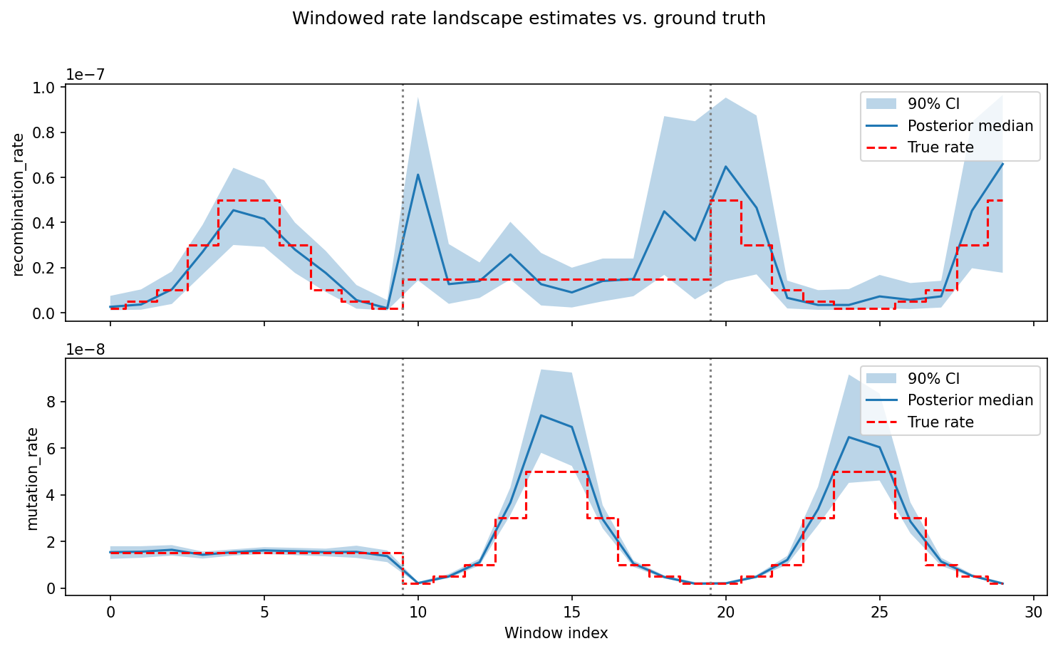
The final result: posterior estimates of recombination rate (top) and mutation rate (bottom) across 30 genomic windows, compared against the true rates used to simulate the example data. Blue shading shows the 90% credible interval; dashed red line is the ground truth. Vertical dotted lines mark chromosome boundaries.
Note
With 5,000 training simulations and the default config, the full
tutorial (training + prediction) takes about 15 minutes on a machine
with an NVIDIA A100 GPU using 4 cores. Simulation is the bottleneck; on
a cluster you can parallelize it further with n_chunk. Training on
CPU will be slower but still feasible.
Prerequisites
Make sure you have installed popgen-npe and activated the environment following the instructions in Installation. All commands below assume the conda environment is active and that you are working from the repository root.
What we are building
Files we will create
─────────────────────
workflow/
├── scripts/
│   └── ts_simulators.py       ← add MutRecRate class here
└── config/
    └── MutRecRate_cnn.yaml    ← new config file

Files shipped with the repo
───────────────────────────
example_data/
└── MutRecRate/
    ├── test.vcf.gz            ← synthetic VCF with variable rates
    ├── test.vcf.gz.tbi
    ├── popmap.yaml
    ├── windows.bed
    └── true_rates.tsv         ← ground truth for comparison
Step 1: Write the simulator
Open workflow/scripts/ts_simulators.py in your favorite editor and add the following class.
The simulator API
Every simulator must:
Inherit from
BaseSimulatorDefine a
default_configdict whose keys are either fixed parameters (single values) or random parameters (two-element[low, high]lists defining uniform prior bounds)In
__init__, buildself.parameters(an ordered list of random parameter names) andself.prior(aBoxUniformover those ranges)Implement
__call__(self, seed) -> (tskit.TreeSequence, np.ndarray)which samples parameters, simulates a tree sequence with mutations, and returns both
Full code listing
class MutRecRate(BaseSimulator):
    """
    Constant-size population with variable mutation and recombination
    rates. Designed for windowed estimation of rate landscapes we train
    on single windows with constant rates, then predict per-window on
    real data.
    """

    default_config = {
        # Fixed parameters
        "samples": {"pop": 20},
        "sequence_length": 500000,
        "pop_size": 10000,
        # Random parameters — [low, high] uniform prior bounds
        "recombination_rate": [1e-9, 1e-7],
        "mutation_rate": [1e-9, 1e-7],
    }

    def __init__(self, config: dict):
        super().__init__(config, self.default_config)
        self.parameters = ["recombination_rate", "mutation_rate"]
        self.prior = BoxUniform(
            low=torch.tensor([self.recombination_rate[0],
                              self.mutation_rate[0]]),
            high=torch.tensor([self.recombination_rate[1],
                               self.mutation_rate[1]]),
        )

    def __call__(self, seed: int = None) -> (tskit.TreeSequence, np.ndarray):
        torch.manual_seed(seed)
        theta = self.prior.sample().numpy()
        recomb_rate, mut_rate = theta

        demography = msprime.Demography()
        demography.add_population(name="pop", initial_size=self.pop_size)

        ts = msprime.sim_ancestry(
            samples={"pop": self.samples["pop"]},
            demography=demography,
            sequence_length=self.sequence_length,
            recombination_rate=recomb_rate,
            random_seed=seed,
        )
        ts = msprime.sim_mutations(ts, rate=mut_rate, random_seed=seed)

        return ts, theta
Key points:
self.parametersdefines the order of values in the returnedthetaarray. This order is used everywhere downstream (training targets, posterior samples, diagnostic plots), so it must be consistent.BoxUniform(fromsbi.utils) is already imported at the top ofts_simulators.py.The population here is named
"pop"(a string, not an integer) — this is required for the prediction pipeline’s population-name matching to work.The
sequence_length(500 kb) matches the window size in the BED file used for prediction. Training windows and prediction windows must be the same size.The prior spans two orders of magnitude (1e-9 to 1e-7), covering the biologically relevant range for most eukaryotes.
Quick sanity check
from workflow.scripts.ts_simulators import MutRecRate

sim = MutRecRate({"class_name": "MutRecRate"})
ts, theta = sim(seed=42)
print(f"Parameters: {dict(zip(sim.parameters, theta))}")
print(f"Num sites:  {ts.num_sites}")
print(f"Num trees:  {ts.num_trees}")
Step 2: Configure the processor
We use the built-in cnn_extract processor, which converts a tree sequence
into a genotype matrix suitable for a convolutional neural network. No new code
is needed here, but one can introduce there own custom processors.
cnn_extract produces an array of shape (2, n_individuals, n_snps) for a
single population. The two channels are SNP positions and genotype values. The
ExchangeableCNN embedding network expects exactly this format.
Key parameters
Parameter |
Meaning |
Our value |
|---|---|---|
|
Maximum number of SNPs to retain |
1000 |
|
Minor allele frequency filter; 0.0 keeps all sites |
0.0 |
|
Whether to keep haplotype-level data (True) or collapse to diploid genotypes (False) |
False |
|
Must be False for |
False |
We use maf_thresh: 0.0 because the full site frequency spectrum
(including rare variants) carries information about the mutation rate.
Step 3: Write the config YAML
Create the file workflow/config/MutRecRate_cnn.yaml with the contents
below. Every field is annotated.
# ── Project location ─────────────────────────────────────────────
# All outputs go under this directory, inside a UID-based
# subdirectory.  Change this to wherever you want results written.
project_dir: "/path/to/your/project/dir"

# ── Resource allocation, if you want to run on a slurm cluster
cpu_resources:
  runtime: "2h"
  mem_mb: 16000

gpu_resources:
  runtime: "4h"
  mem_mb: 50000
  gpus: 1
  slurm_partition: "gpu"
  slurm_extra: "--gres=gpu:1"

# ── Simulation settings ──────────────────────────────────────────
random_seed: 42
n_chunk: 10          # number of parallel simulation jobs
n_train: 5000        # training simulations
n_val: 500           # validation simulations
n_test: 500          # test simulations (used for diagnostics)

# ── Training hyperparameters ─────────────────────────────────────
train_embedding_net_separately: True   # two-stage training
use_cache: True                        # load features into CPU memory
optimizer: "Adam"
batch_size: 64
learning_rate: 0.0005
max_num_epochs: 200
stop_after_epochs: 50       # early stopping patience
clip_max_norm: 5
packed_sequence: False

# ── Simulator ────────────────────────────────────────────────────
# class_name must match the class you added to ts_simulators.py.
# sequence_length must equal the window size in the BED file.
simulator:
  class_name: "MutRecRate"
  samples:
    pop: 20
  sequence_length: 500000
  pop_size: 10000

# ── Processor ────────────────────────────────────────────────────
processor:
  class_name: "cnn_extract"
  n_snps: 1000
  maf_thresh: 0.0

# ── Embedding network ────────────────────────────────────────────
# input_rows: number of individuals per population (list, one per pop)
# input_cols: number of SNPs per population (list, one per pop)
embedding_network:
  class_name: "ExchangeableCNN"
  output_dim: 64
  input_rows: [20]
  input_cols: [1000]

# ── Prediction ───────────────────────────────────────────────────
prediction:
  n_chunk: 5
  vcf: "example_data/MutRecRate/test.vcf.gz"
  population_map: "example_data/MutRecRate/popmap.yaml"
  windows: "example_data/MutRecRate/windows.bed"
  min_snps_per_window: 10
What are all these yaml fields anyway? Some explanation:
project_dir— the workflow creates a subdirectory namedMutRecRate-cnn_extract-ExchangeableCNN-42-5000-sepunder this path (the naming scheme is{simulator}-{processor}-{embedding}-{seed}-{n_train}-{sep|e2e}).n_chunkcontrols parallelism. Withn_train: 5000andn_chunk: 10, each chunk simulates 500 tree sequences. On a laptop,n_chunk: 1or2is fine; on a cluster you can go much higher.train_embedding_net_separately: Truemeans the CNN embedding is pre-trained, then the normalizing flow is trained on the learned embeddings. This is can be more stable than end-to-end training.sequence_length: 500000— this must match the window size inwindows.bed. Training windows and prediction windows must be the same size so the network sees the same scale of data.input_rowsandinput_colsmust match the processor output: 20 individuals and 1000 SNPs.
Step 4: Run the training workflow
From the repository root:
snakemake \
    --configfile workflow/config/MutRecRate_cnn.yaml \
    --snakefile workflow/training_workflow.smk \
    --cores 4
Tip
On a local machine with no GPU, training will still work (PyTorch falls back to CPU) but will be slower. With 5,000 training simulations and the network sizes above, expect roughly 10–30 minutes depending on your machine.
What happens
The workflow runs these stages in order:
Setup — creates the Zarr data store and divides the simulations into chunks.
Simulate — each chunk calls
MutRecRate(seed=...)repeatedly, drawing random rate pairs from the prior and simulating constant-rate windows.Process — each chunk calls
cnn_extracton every tree sequence, storing the resulting tensors in Zarr.Train embedding network — trains the
ExchangeableCNNto produce useful summary statistics from genotype matrices.Train normalizing flow — trains a neural posterior estimator conditioned on the learned embeddings.
Diagnostics — generates posterior calibration, concentration, and simulation summary plots.
Output files
After a successful run you will find (under your project_dir):
MutRecRate-cnn_extract-ExchangeableCNN-42-5000-sep/
├── tensors/zarr/                    # Zarr store with features and targets
├── trees/                           # Simulated tree sequences (.trees)
├── logs/                            # TensorBoard training logs
├── pretrain_embedding_network       # Pickled trained CNN
├── pretrain_normalizing_flow        # Pickled trained flow
└── plots/
    ├── posterior_calibration.png
    ├── posterior_concentration.png
    ├── posterior_expectation.png
    ├── posterior_at_prior_mean.png
    ├── posterior_at_prior_low.png
    ├── posterior_at_prior_high.png
    ├── simulation_stats.png
    ├── stats_vs_params_pairplot.png
    └── stats_heatmaps.png
Inspecting results
The diagnostic plots are the quickest way to check that inference is working:
posterior_calibration.png — simulation-based calibration plot; points falling on the diagonal indicate well-calibrated posteriors.
posterior_concentration.png — shows how ratio of posterior to prior width change as a function of coverage for each parameter.
posterior_expectation.png — posterior means vs. true parameter values; points near the diagonal mean the model is recovering the parameters.
posterior_at_prior_mean.png / _low.png / _high.png — posterior distributions evaluated at specific points in the prior (mean, lower bound, upper bound), useful for spotting bias at the edges of the parameter space.
simulation_stats.png — summary statistics of the simulated datasets.
stats_vs_params_pairplot.png — pairwise relationships between simulation summary statistics and the underlying parameters.
stats_heatmaps.png — heatmaps showing correlations between summary statistics and parameters.
You can also monitor training loss in real time with TensorBoard:
tensorboard --logdir /path/to/your/project/dir/MutRecRate-cnn_extract-ExchangeableCNN-42-5000-sep/logs
Step 5: Run prediction on the example data
The prediction workflow applies your trained model to genomic data stored in VCF format, producing windowed posterior estimates across the genome.
The bundled example data in example_data/MutRecRate/ contains a synthetic
VCF simulated with spatially varying recombination and mutation rates across
three chromosomes (5 Mb each, 10 windows of 500 kb per chromosome). This lets
you verify that the trained model recovers the known rate landscape.
The example data includes:
test.vcf.gz — simulated with
msprime.RateMapobjects so that rates vary across windows (e.g., chr0 has varying recombination but constant mutation; chr1 has varying mutation but constant recombination; chr2 has both varying in opposite directions).popmap.yaml — maps all 20 VCF samples to population
"pop".windows.bed — 30 windows (10 per chromosome, 500 kb each).
true_rates.tsv — ground truth recombination and mutation rates per window, for comparison with the model’s predictions.
Requirements for prediction data
If you are bringing your own data instead of using the example, note:
The VCF must be bgzipped and tabix-indexed.
Every contig must have a length in the VCF header (
##contig=<ID=...,length=...>). If contig lengths are missing,tsinferwill fail withsequence_length cannot be zero or less.The number of samples in the VCF (after filtering via the population map) must exactly match the simulator’s
samplesconfig — in our case, 20 diploid individuals assigned to population"pop".Window sizes in the BED file should match the simulator’s
sequence_length.
The population map assigns VCF sample names to simulator population names:
# popmap.yaml
IND0: "pop"
IND1: "pop"
IND2: "pop"
# ... one entry per VCF sample
Run the prediction workflow
The prediction block is already in the config from Step 3. Run:
snakemake \
    --configfile workflow/config/MutRecRate_cnn.yaml \
    --snakefile workflow/prediction_workflow.smk \
    --cores 4
What the prediction workflow does
Convert VCF — converts the bgzipped VCF to Zarr format (
vcf2zarr).Setup — validates that VCF samples match the simulator, defines windows, and creates Zarr storage.
Infer trees — for each window, infers a tree sequence from the genotype data using
tsinfer.Process — applies the same
cnn_extractprocessor to each inferred tree sequence.Predict — loads the trained embedding network and normalizing flow, and draws 1,000 posterior samples per window.
Diagnostics — generates summary plots.
Prediction output
test.vcf.gz/
├── vcz/                    # Zarr-encoded VCF
├── trees/                  # Inferred tree sequences (one per window)
├── tensors/zarr/           # Features and posterior samples
│   └── predictions         # Shape: (n_windows, n_parameters, 1000)
└── plots/
    ├── posteriors-across-windows.png
    └── tree_stats_hist.png
posteriors-across-windows.png — a heatmap showing the posterior distribution for each parameter across all 30 genomic windows. This is the main result: you should see the posterior mode tracking the true rate landscape across windows and chromosomes (separated by red dashed lines).
tree_stats_hist.png — summary statistics of the inferred tree sequences compared with simulated training data, useful for checking that the real data falls within the range the model was trained on.
Step 6: Interpret the results
The raw posterior samples are stored in tensors/zarr/predictions as a
NumPy array of shape (n_windows, n_parameters, 1000). You can load them
for downstream analysis and compare against the known ground truth:
import zarr
import numpy as np
import matplotlib.pyplot as plt

# Load predictions and ground truth
project = "/path/to/your/project/dir/MutRecRate-cnn_extract-ExchangeableCNN-42-5000-sep"
predictions = zarr.load(f"{project}/test.vcf.gz/tensors/zarr/predictions")
true_rates = np.loadtxt("example_data/MutRecRate/true_rates.tsv",
                        skiprows=1, usecols=[3, 4])

param_names = ["recombination_rate", "mutation_rate"]
fig, axes = plt.subplots(2, 1, figsize=(10, 6), sharex=True)
for i, (ax, name) in enumerate(zip(axes, param_names)):
    # Plot posterior medians and 90% credible intervals
    medians = np.median(predictions[:, i, :], axis=1)
    lo = np.quantile(predictions[:, i, :], 0.05, axis=1)
    hi = np.quantile(predictions[:, i, :], 0.95, axis=1)
    windows = np.arange(predictions.shape[0])
    ax.fill_between(windows, lo, hi, alpha=0.3, label="90% CI")
    ax.plot(windows, medians, label="Posterior median")
    ax.step(windows, true_rates[:, i], where="mid",
            color="red", linestyle="--", label="True rate")
    ax.set_ylabel(name)
    ax.legend(loc="upper right")
    # Mark chromosome boundaries
    for b in [10, 20]:
        ax.axvline(b - 0.5, color="gray", linestyle=":")
axes[-1].set_xlabel("Window index")
plt.tight_layout()
plt.savefig("rate_landscape_comparison.png", dpi=150)
Next steps
Try log-scale priors — rates spanning orders of magnitude are more naturally modeled with log-uniform priors. You could sample in log space (e.g.,
log10_recomb_rate: [-9, -7]) and exponentiate inside__call__, similar to theVariablePopulationSizesimulator.Try different architectures — swap
cnn_extract/ExchangeableCNNforgenotypes_and_distances/RNN, or use summary statistics withtskit_sfs/SummaryStatisticsEmbedding. See the processor–network compatibility table for valid combinations.Explore existing configs — the
workflow/config/directory has examples for multi-population models (YRI_CEU_cnn.yaml), variable population size (variable_popnSize_spidna.yaml), and more.Scale up — increase
n_trainandn_chunkfor better inference, and use SLURM resource blocks for cluster execution. See Usage for details.Consult the API reference — Simulators and Processors document every built-in class, their parameters, and their configuration options.